|
0 Comments
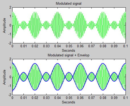 A=0.5; t=0:0.0001:1; modulatedSignal=[A+cos(2*pi*50*t)].*cos(2*pi*1000*t); subplot(2,1,1); plot(t,modulatedSignal,'g'); set(gca,'xlim',[0 0.1]); title('Modulated signal'); xlabel('Seconds'); ylabel('Amplitude'); y=hilbert(modulatedSignal); envelop=abs(y); subplot(2,1,2) plot(t,modulatedSignal,'g'); hold on; plot(t,envelop,'b','linewidth',2); plot(t,-envelop,'b','linewidth',2); title('Modulated signal + Envelop'); xlabel('Seconds'); ylabel('Amplitude'); set(gca,'xlim',[0 0.1]); 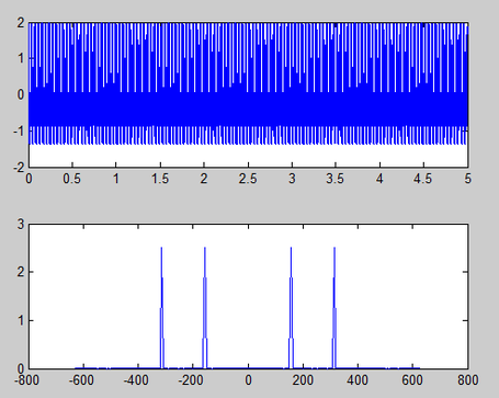 t=0:0.001:5;
f=zeros(size(t)); for i=1:length(t) if abs (t(i)-5)<=0.5; f(i)=1; else f(i)=0; end end f=cos(50.*pi.*t); f=sin((100*pi*t)+(pi/3)); f=cos(50.*pi.*t)+sin((100*pi*t)+(pi/3)); subplot(2,1,1) plot(t,f,'linewidth',2) w=[-50:1:50]; w=[-200*pi:2*pi:200*pi] F=zeros(size(w)); for k=1:length(w) F(k)=trapz(t,f.*exp(-j*w(k)*t)); end F_mag=abs(F); subplot(2,1,2) plot(w,F_mag) t1=-pi:0.001:0;%time index y1=-2;%defining signal mathematically t2=0:0.001:pi;%time index y2=1;%defining signal mathematically t=[t1 t2]; y=[(-2)*ones(size(t1)) (1)*ones(size(t2))]; subplot(2,2,1) plot(t,y) title('origional signal') a0=1/(2*pi)*trapz(t,y);%integration of y w.r.t to t for n=1:1:7 %calculating first seve values y1=y.*cos(n*t);%w=2 an(n)=(2/(2*pi))*trapz(t,y1); y2=y.*sin(n*t);%multiplication value by value bn(n)=(2/(2*pi))*trapz(t,y2); end w=1:1:7; cn1=(an.^2)+(bn.^2);%magnitude cn=sqrt(cn1);%taking square root subplot(2,2,2); stem(w,cn) title('magnitude plot of fourier series of origional signal') theta=atan(-bn./an);%for phase subplot(2,2,3) stem(w,theta); title('phase plot of fourier series of origional signal') for u=1:1:7 a=cn(u)*cos((2*u*t)+theta(u)); end g=a0+a; subplot(2,2,4) stem(t,g) title('the final signal g(t)') 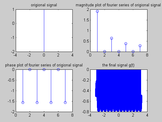
t=-pi:0.001:pi;%time index y=t;%defining signal mathematically subplot(2,2,1) plot(t,y) title('origional signal') a0=1/(2*pi)*trapz(t,y);%integration of y w.r.t to t for n=1:1:7 %calculating first seve values y1=y.*cos(n*t);%w=1 an(n)=(2/(2*pi))*trapz(t,y1); y2=y.*sin(n*t);%multiplication value by value bn(n)=(2/(2*pi))*trapz(t,y2); end w=1:1:7; cn1=(an.^2)+(bn.^2);%magnitude cn=sqrt(cn1);%taking square root subplot(2,2,2); stem(w,cn) title('magnitude plot of fourier series of origional signal') theta=atan(-bn./an);%for phase subplot(2,2,3) stem(w,theta); title('phase plot of fourier series of origional signal') for u=1:1:7 a=cn(u)*cos((2*u*t)+theta(u)); end g=a0+a; subplot(2,2,4) stem(t,g) title('the final signal g(t)') 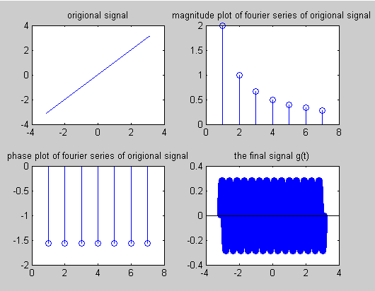
t=0:0.001:pi;%time index y=exp(-t/2);%defining signal mathematically subplot(2,2,1) plot(t,y) title('origional signal') a0=1/pi*trapz(t,y);%integration of y w.r.t to t for n=1:1:7 %calculating first seve values y1=y.*cos(2*n*t);%w=2 an(n)=(2/pi)*trapz(t,y1); y2=y.*sin(2*n*t);%multiplication value by value bn(n)=(2/pi)*trapz(t,y2); end w=1:1:7; cn1=(an.^2)+(bn.^2);%magnitude cn=sqrt(cn1);%taking square root subplot(2,2,2); stem(w,cn) title('magnitude plot of fourier series of origional signal') theta=atan(-bn./an);%for phase subplot(2,2,3) stem(w,theta); title('phase plot of fourier series of origional signal') for u=1:1:7 a=cn(u)*cos((2*u*t)+theta(u)); end g=a0+a; subplot(2,2,4) stem(t,g) title('the final signal g(t)') 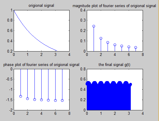 V=10; %the peak voltage
f0 = 1; % Fundamental frequency in Hertz w0 = 2*pi*f0; % Fundamental frequency in radians T=1/f0; % the period of the square wave V=5; %the peak voltage
f0 = 1000; % Fundamental frequency in Hertz w0 = 2*pi*f0; % Fundamental frequency in radians T=1/f0; % the period of the square wave |
Categories
All
Archives
March 2014
This section will not be visible in live published website. Below are your current blog design settings: Current Number Of Columns are = 1 Blog Post Style = card Use of custom card colors instead of default colors = Blog Post Card Background Color = current color Blog Post Card Shadow Color = current color Blog Post Card Border Color = current color Use of custom colors instead of theme colors for below options= Blog Post Title Color = current color Blog Post Title Hover Color = current color Blog Post Date Color = current color Blog Post Date Hover Color = current color Blog Post Read More Link Color = current color Blog Post Read More Link Hover Color = current color Blog Post Comments Count Color = current color Blog Post Comments Count Hover Color = current color |
 RSS Feed
